The performance distribution in your organisation is not the one you think it is

Why the performance distribution you observe tells you almost nothing about the one that actually exists.

A few weeks ago I read a Substack article by Colby Kennedy Nesbitt titled “Is Performance a Power Law?” which I recommend. She makes a careful and important distinction: the claim that job performance follows a power law - that the top 20% of employees do 80% of the work - rests on a confusion between performance outputs and the underlying capability that produces them. The outputs of performance (home runs, sales figures, publications) can follow a power law for structural reasons that have nothing to do with the shape of human capability. Count metrics are bounded at zero and unbounded above. They are shaped by exposure time, opportunity, and attribution, not just ability. When you normalise for those factors - when you move from home runs to slugging percentage, say - the distribution tightens towards something closer to normal.

“Performance is not a power law. Some performance outputs are. Confusing the two warps how we measure, reward, and develop.”

“The shape of the distribution shifts with the structure of the metric, not the nature of performance itself.”

• Colby Kennedy Nesbitt, Is Performance a Power Law?

I should confess here that I know almost nothing about baseball. I encountered the game analytically, through David Robinson’s excellent book on Empirical Bayes estimation, not through watching it. Slugging percentages entered my vocabulary as illustrative examples rather than as statistics I track on weekends. This is perhaps fitting for an article about European HR practitioners importing ideas from American I/O psychology with imperfect understanding of their original context.

Nesbitt’s argument is convincing as far as it goes. But I found myself stopping at a particular line and thinking: this is where the interesting problem begins, not where it ends. Even if we accept - as I do - that the underlying distribution of human performance capability is approximately normal, the distribution of performance we observe inside any organisation tells us almost nothing about that underlying distribution. The two are separated by a set of processes that are systematic, cumulative, and poorly understood. And worse, the effect of those processes is to make the observed distribution look more normal than it should - which means the standard assumption appears to be confirmed precisely because the measurement system is producing the artefact.

That is what this article is about.

---

What are we measuring? Two disciplines, two answers

I came to People Analytics as an economist, which shapes how I think about performance in ways I have only gradually become conscious of. When economists study performance, they are studying output - the value a worker contributes to the firm, net of the cost of employing them. Productivity, in the economic sense, is the marginal revenue product of labour. It is an economic construct, defined against a market, not against a behaviour taxonomy. When the economist thinks of labour as being substitutable by capital, freelancers, management consultants or now AI it’s this view of performance which lets us do so.

I/O psychology, which is the academic discipline that has shaped HR practice, starts from a completely different place. John Campbell, in a foundational paper in 1990, defined job performance as behaviour under an individual’s control that contributes to organisational goals - not outputs, but the behaviours that produce outputs. His taxonomy identifies eight dimensions including task proficiency, demonstrating effort, facilitating peer performance, and maintaining personal discipline. By this definition, performance is multi-dimensional, hierarchical, and largely behavioural. The downstream result of that performance - revenue, publications, home runs - is not performance; it is a consequence of performance.

This is not academic hair-splitting. The distinction matters for how organisations measure, reward, and manage. When HR collapses eight dimensions of performance into a single annual rating, it is doing something that neither the economic framework nor the I/O psychology framework endorses. The economist wants to know the marginal revenue product; the rating doesn’t tell them that. The I/O psychologist wants to measure behavioural proficiency on multiple independently weighted dimensions; the rating collapses those into a spurious single number.

George Baker, in a 1992 paper in the Journal of Political Economy, put this with characteristic precision. Any measurable proxy for performance will systematically diverge from the underlying construct the firm actually cares about. He called this distortion. If you pay mechanics based on completed repairs, you create an incentive to recommend unnecessary ones - because the thing you can count is not the same as the thing you value. Bengt Holmström and Paul Milgrom showed in 1991 that this problem is structurally insoluble when workers have multiple tasks and only some are measurable: performance pay on the measurable tasks will divert effort away from the unmeasurable ones, which may be exactly the ones that matter most.

I think about this often in relation to certain financial roles. A derivatives trader who is paid on the mark-to-market value of her book at point of sale has every incentive to maximise initial pricing at the cost of longer-term performance on the instrument. Her current performance metric is excellent. Her expected future contribution to the firm - the present discounted value of all the outcomes her decisions will eventually produce - may be negative. Performance management systems that are backward-looking are not measuring the thing that matters; they are measuring a time-limited proxy for it, one that rational agents will optimise at the expense of the real thing.

---

The distribution debate: what we actually know

Against this backdrop, the argument about whether performance follows a normal or power-law distribution takes on a slightly different character. The debate is real, and it matters practically. But it is also somewhat harder to resolve than either camp acknowledges.

Ernest O’Boyle and Herman Aguinis made the power-law case in a 2012 paper in Personnel Psychology, drawing on 198 samples and over 633,000 individuals across research, entertainment, politics, and sport. They found that individual performance consistently fitted a Paretian distribution better than a normal one. The implication they drew - and that subsequently escaped into HR practice as a management principle - was that the top performers are so much better than the rest that entire compensation philosophies should be reoriented around them.

Joel Beck, Alexander Beatty, and Paul Sackett responded in 2014 with a careful methodological critique. Their key demonstration was that sampling from only the upper tail of a normal distribution - which is precisely what populations of elite researchers, athletes, and entertainers are - produces highly skewed data even when the underlying distribution is perfectly normal. The apparent power law may be a property of sample selection rather than of human capability.

Nesbitt adds the metric structure argument I described in the opening. Count statistics (publications, home runs) have structural properties - bounded at zero, unbounded above, shaped by opportunity - that generate skew regardless of the underlying ability distribution. When you normalise for those structural features, the skew largely disappears.

I find both the Beck et al. and Nesbitt arguments convincing. But I want to add a third layer, which neither addresses: the sample that organisational performance management is observing is not the kind of sample from which distributional conclusions can reliably be drawn.

---

The sample you cannot see

Here is the problem in its simplest form. Any claim about the distribution of performance within a firm implicitly assumes that the employees you are observing constitute a meaningful sample from the population you care about. They do not. They are the survivors of at least four sequential selection processes, each applied with substantial measurement error, each systematically biasing who remains.

Stage 1: Selection at entry. The firm applies a selection procedure to an applicant pool. Even a good one - a procedure with validity around 0.40, which is high by real-world standards - leaves substantial error. The hired cohort is range-restricted: those below the selection threshold are absent. That threshold is itself applied to a noisy score, so some of the people below the threshold in terms of true capability were hired anyway, and some above it were not. From the first day of employment, the in-firm distribution is not a random draw from the labour market. But it is also not a pure ‘sampling from the upper tail’ because you have the measurement error of selection.

Stage 2: Differential voluntary attrition. Workers leave at different rates correlated with their ability. High-capability employees have more outside options - their ability is visible to other employers through the labour market signalling process - and so they leave at higher rates. But there is a second, subtler mechanism at work that I have observed consistently in organisations, especially those with structured bonus programmes. Employees join with expectations about their career trajectory: not just their starting salary but the expected value of their development over time, discounted for risk. When the firm’s annual signals - the rating, the bonus allocation - fall short of those expectations, the employee updates their belief about whether this firm will help them develop as they hoped. If the gap is large enough, they start looking elsewhere.

This second mechanism has a particularly perverse interaction with measurement error. Under the first mechanism, the people who leave are genuinely high-ability - the firm loses people it wants to keep, but at least the cause is structural (the market). Under the second mechanism, the people who leave are those who received signals below their expectations. With imperfect measurement, that includes high-ability employees who were rated low through inter-rater noise. The firm does not know these were its best performers, because the rating that prompted them to leave was itself wrong. Meanwhile, lower-ability employees who were fortunate enough to receive inflated ratings stay longer than they should, because the firm’s signal confirmed their self-assessment.

Stage 3: Performance management out. Firms explicitly remove workers at the lower end of their performance distribution. Probationary dismissals, performance improvement plans, and redundancy selection all systematically truncate the lower tail. The criterion used is measured performance - which, as I will show in the simulation, carries a noise component that is roughly as large as the true signal. Some genuinely low-performing employees are removed correctly. Some higher-performing employees who received a bad rating in a bad year are removed incorrectly. The resulting sample is not “everyone above the true performance threshold.” It is everyone above a noisy, error-prone estimate of that threshold.

Stage 4: Retention interventions. Firms apply retention tools - above-market pay, bonus guarantees, high-visibility assignments - disproportionately to employees they believe are high performers. Those beliefs are, again, based on measured performance. So the upper tail of the distribution is partially rebuilt through a process that has the same measurement error as everything else.

After five years of this, the distribution of performance ratings in a firm reflects something that is genuinely complex: the joint operation of market dynamics, firm policies, and measurement error on whatever the true underlying distribution is. James Heckman won the Nobel Prize in Economics in 2000 partly for developing formal methods to correct for this kind of endogenous sample selection. His point was that estimates from selected samples are biased in ways that are not visible from within the sample itself - you cannot identify the selection bias from the selected data alone. That applies directly to performance distributions.

The insight from psychometrics is adjacent: range restriction - the well-documented consequence of selecting a non-random subset of the population - attenuates the observed variance and distorts correlations. Corrections for indirect range restriction (where selection happens on a variable correlated with, but not identical to, the criterion of interest) are standard in meta-analyses of selection validity. They are rarely applied when interpreting performance distributions.

---

Noise and bias: the measurement problem HR gets backwards

There is a further dimension to the measurement problem that I think the HR profession has consistently misunderstood, and it requires a brief detour into Daniel Kahneman, Olivier Sibony, and Cass Sunstein‘s 2021 book Noise: A Flaw in Human Judgment.

The way HR talks about measurement error in performance ratings is almost entirely a conversation about bias. Leniency bias - managers who rate too generously. Severity bias - managers who rate too harshly. Halo effects, recency bias, demographic biases. Vast effort goes into calibration sessions designed to align rating distributions across managers and reduce systematic distortions. The underlying assumption is that the core problem with performance ratings is that they are systematically skewed in a predictable direction.

Kahneman, Sibony, and Sunstein argue that this focus is importantly incomplete. Bias is systematic error - it shifts ratings in a consistent direction and can, in principle, be identified and corrected. Noise is something different: it is the random, unsystematic variability in judgements that has nothing to do with the person being rated. The same manager assessing the same employee on a different day, or two different managers assessing the same employee, produce different ratings for reasons that are effectively random. Their core finding, demonstrated across multiple domains of professional judgement including medical diagnosis, legal sentencing, and credit assessment, is that noise is typically larger than bias in absolute magnitude.

For performance ratings, this matters in a specific way. Calibration sessions address bias - they bring systematic leniency and severity into alignment. They do almost nothing about noise. The manager who rates consistently harsh can be corrected. The manager who rates differently on different days, or whose assessment varies unpredictably depending on their mood, the order in which they reviewed employees, or the ambient light in the room cannot be corrected without measuring the same employee multiple times by multiple raters and averaging the result. That is not how annual performance reviews work.

When Frank Schmidt and John Hunter established that inter-rater reliability for performance ratings is approximately 0.52 across the meta-analytic evidence base, they were quantifying noise as much as bias. At that level of reliability, roughly half the variance in any performance rating is random error. The HR profession’s focus on bias over noise has a practical consequence: it addresses the smaller part of the measurement problem while leaving the larger part untouched. The noise is not a detail. It is half the data.

---

Introducing PQ: a simulation device

To explore these dynamics, I want to introduce a modelling tool. I am going to call it PQ - Performance Quotient. Like IQ, PQ is assumed to be normally distributed in the general working population: mean 100, standard deviation 15. It represents the latent capability underlying performance behaviour. I am not claiming PQ exists as a real, measurable construct. I am using it as a device - a clean, understandable baseline - to ask: what happens to a normal distribution when you run it through an organisation’s HR processes?

The device also helps me be explicit about what I am assuming. Starting with normally distributed PQ is a deliberate charitable premise: even granting the normality assumption, I want to show that what the organisation observes will not be normal, and more importantly, that the observed distribution cannot be used to infer the true one.

Before showing the results, I want to explain why I think simulation is the right tool for this problem, because I believe it is underused as a thinking practice in HR and People Analytics - and in business more broadly.

The argument I have been making in the preceding sections is hard to hold in your head all at once. Four selection stages, each with its own error rate, operating on an unknown true distribution, compounding over five years - the verbal argument can gesture at this, but it cannot make you feel the scale of the distortion. The standard intuition that “a big enough sample reveals the true distribution” fails here precisely because the sample is itself the product of the processes we are trying to understand. More data does not help; the data is the problem.

Simulation forces a different kind of clarity. You must make your assumptions explicit. You cannot write “differential attrition” as a vague phrase and then proceed; you have to specify a quit probability function, decide whether it responds to true PQ or measured PQ or the gap between career expectations and the firm’s signals, and commit to numbers. That process of commitment is epistemically valuable - it reveals where your argument depends on assumptions you have not examined, and where it holds across a wide range of plausible values.

In my experience, the standard research process in People Analytics goes: question → data collection → statistical analysis → conclusion. The simulation step - which would sit between question and data collection, asking “what would we expect to find if the mechanism we are hypothesising were actually operating?” - is almost always skipped. The result is that practitioners often lack a strong prior about what the data should look like before they examine it, which makes interpretation harder and increases the risk of finding patterns that confirm prior beliefs rather than testing them. A simulation built before looking at the data is one of the few tools that can genuinely discipline that process.

---

What the simulation shows

I ran a simulation in R across five annual cycles, hiring from a pool of 1,000 applicants each year at a 20% selection rate, applying a realistic selection procedure (validity 0.40), differential attrition by PQ rank, performance management of the bottom 5% annually, and targeted retention bonuses for high performers.

Figure 1 shows Stage 1: no measurement error, policies applied with perfect information apart from the selection procedure. Even under these idealised conditions, the in-firm PQ distribution diverges substantially from the population within two years. At hire, selection has already truncated the lower tail. By Year 5, the combined effect of performance management, differential attrition, and retention interventions has produced a distribution that is visibly non-normal: a steep left wall, a sharpened and compressed peak, an asymmetric shape bearing little resemblance to the underlying population. With perfect measurement, the distortion is apparent to anyone who looks. The uncomfortable implication follows in Figure 2 - with realistic measurement error, that distorted shape becomes much harder to see. I'd argue we might want a distribution like Year 5, but it's certainly not a normal distribution. It’s close but not the same as Beck, Beaty, and Sackett’s sample.

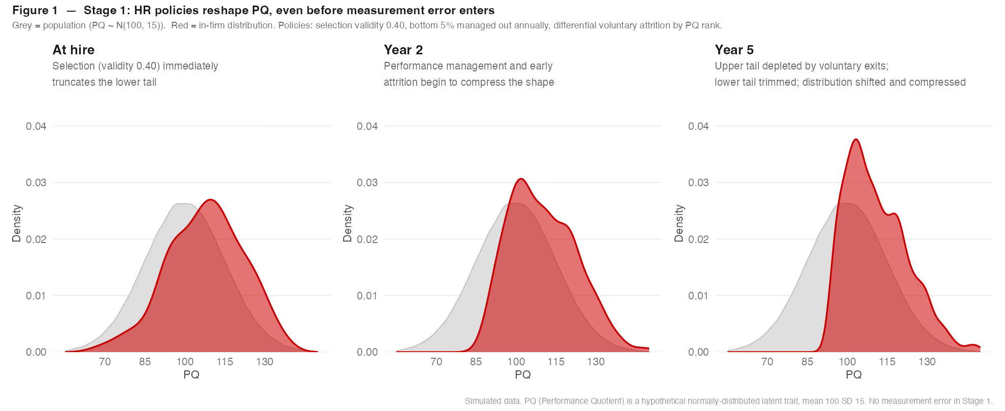
Figure 2 adds measurement error at the meta-analytic inter-rater reliability of 0.52, the figure Frank Schmidt and John Hunter established across decades of careful research. At this level of reliability, the standard deviation of measurement error is approximately 14.4 PQ points - almost as large as the true standard deviation of 15. Half the variance in any performance rating is noise.

The comparison across three panels is the core of the article’s argument. The left panel shows the Stage 1 Year 5 distribution - the best possible world, with perfect measurement. The centre panel shows what Stage 2 does to the true PQ distribution: measurement error causes false exits (high-PQ employees misrated low and managed out, or misrated low and therefore disappointed in their career signal, who then leave) and false retentions (low-PQ employees misrated high who stay). Actual workforce quality is worse than it would be with better measurement.

The right panel is the one that I find most striking. It shows not the true PQ distribution but the observed performance rating distribution - what HR actually sees when it looks at its data. The noise has recreated a distribution with fatter tails than the normal. The truncations and compressions in the true distribution have been smoothed over by the random error in the ratings. The bell curve in the data is not evidence that the true distribution is normal. It may be evidence that the measurement error is large enough to obscure a distribution that is not normal.

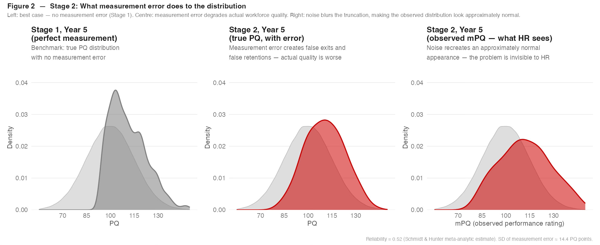
Figure 3 separates the two attrition mechanisms. The left panel shows a world where only Mechanism A operates - high-PQ employees leave because they have better options. The right panel adds Mechanism B: employees in bonus-structured firms who receive signals below their career expectations leave regardless of their absolute performance level. The combined effect is more severe, and its character is different. Mechanism A depletes the upper tail of the true PQ distribution in a relatively predictable way. Mechanism B creates a compound adverse selection problem: the firm loses some of its best people because its own measurement told them they were not valued, while retaining mediocre employees whose inflated ratings kept them satisfied.

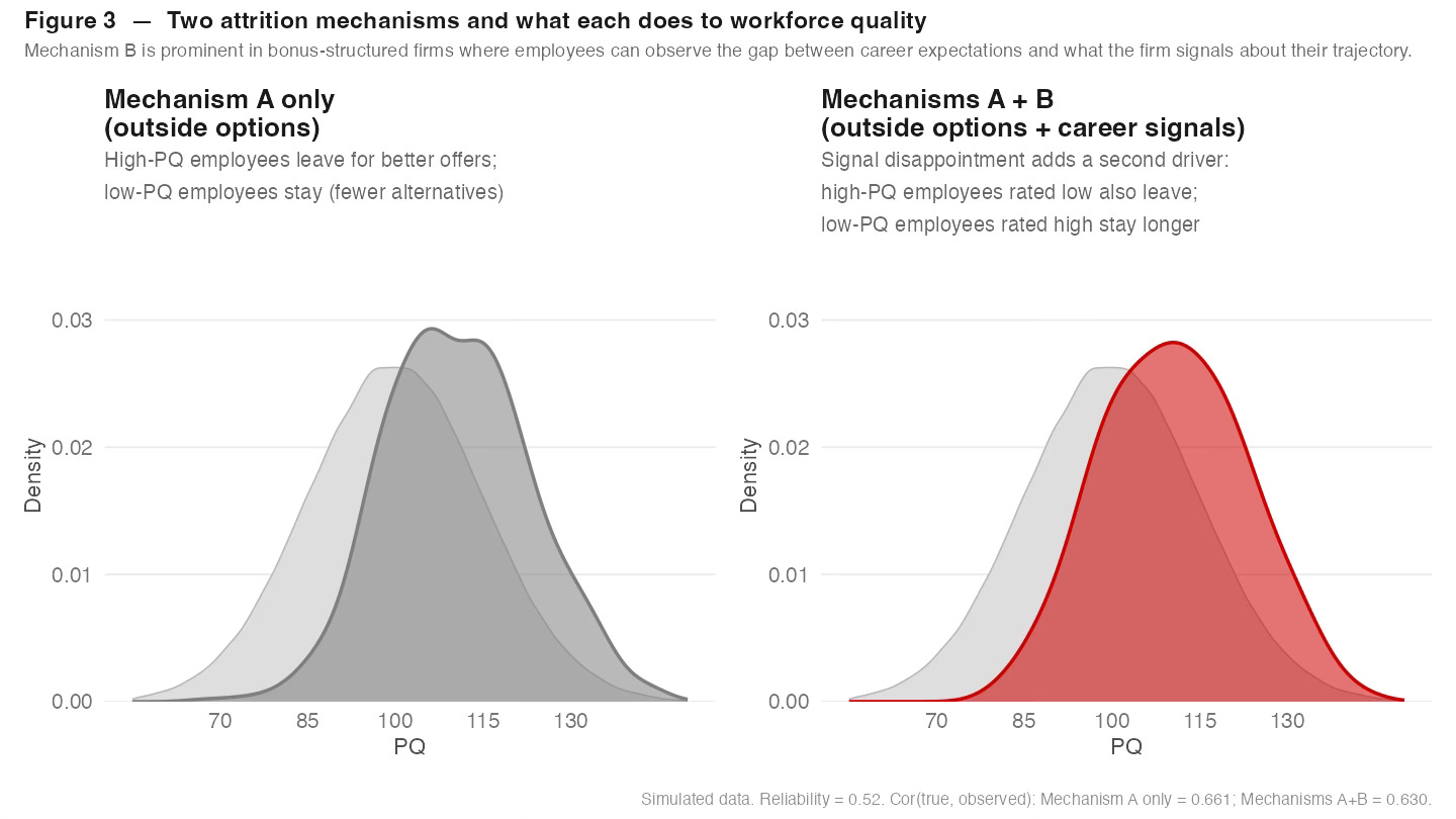
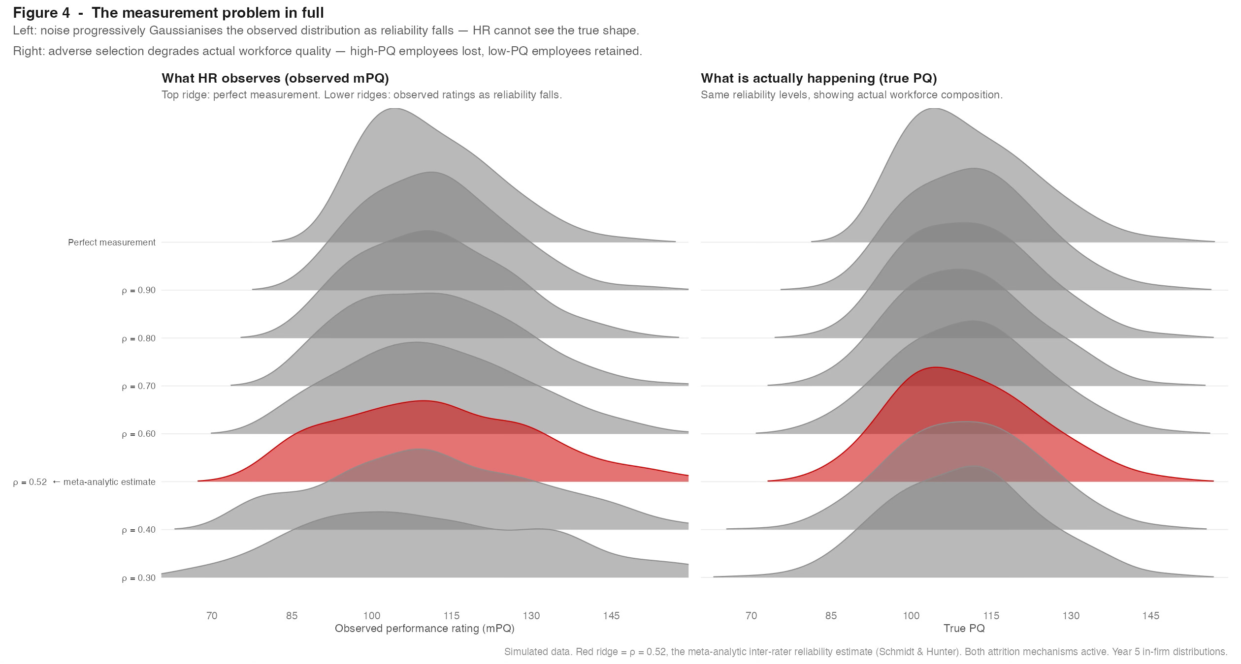
Figure 4 shows what happens across a range of reliability values, from 0.30 at the bottom to near-perfect measurement at the top. The two panels tell different stories about the same simulation.

The left panel shows the observed mPQ distribution - what HR actually sees in its rating data at each reliability level. The striking result is how quickly the distribution collapses toward something that looks approximately normal and then past it. At reliability of 0.52, the clean left-truncation visible in Figure 1 has largely disappeared. But this is not evidence that the organisation has become a random sample of the population. It is evidence that the cumulative noise in annual ratings has grown large enough to overwrite the signal. Five years of selection, performance management, and differential attrition have shaped the true distribution substantially - but the observed rating distribution makes it appear as if almost none of that has happened. The observed mPQ distribution at realistic reliability levels most closely resembles the at-hire distribution from Year 1, before any of those processes have run. The HR processes are doing work; the measurement system is hiding it.

There is a second, subtler effect visible in the left panel. HR does not just see a distribution that looks more normal than it should. It sees one with somewhat thicker tails - more apparent high performers and more apparent low performers than actually exist, at the expense of the proportion near the centre. This is noise doing what noise does: redistributing people away from their true score in both directions. The employee rated in the bottom 5% is not reliably a low performer. The employee rated in the top 10% is not reliably exceptional. At an inter-rater reliability of 0.52, a substantial fraction of both groups are there by measurement accident rather than genuine performance.

The right panel shows the true PQ distribution at the same reliability levels - what HR cannot see. As reliability falls, actual workforce quality deteriorates. Fewer high-PQ employees survive the combined effect of false low ratings, which push some of the best out through performance management or career disappointment, and false high ratings, which protect some of the weakest from scrutiny. The organisation believes, from its rating data, that it is managing performance actively. It is - but with a large fraction of its effort directed at the wrong people.

---

What follows from this

I want to be careful about what I am and am not claiming. The simulation is illustrative - it uses parameters chosen to be plausible and instructive, not to reproduce any specific organisation. Different organisations will have different selection validity, different attrition patterns, different reliability in their rating processes. The purpose of the simulation is to show the mechanism - to demonstrate that even under generous assumptions, the four-stage HR process systematically reshapes the in-firm distribution in ways that make it uninformative about the true underlying distribution.

The practical implications are uncomfortable but clear. Organisations that use forced distribution curves - requiring managers to rate a fixed percentage of employees as top, middle, and bottom performers - are imposing a distributional assumption on a sample that has already been shaped by that same assumption in previous years. The policy creates a feedback loop: managing out low performers changes the distribution, which changes who the “low performers” are in the next cycle, which changes the distribution again. This is not a bell curve naturally occurring in the workforce. It is a bell curve that the organisation’s own processes are manufacturing and then observing with satisfaction.

There is a further problem that becomes visible once you take noise seriously. The employees rated in the bottom 5% of the observed distribution are not all genuinely low performers. At inter-rater reliability of 0.52, with measurement error of roughly the same magnitude as the true signal, the bottom of the rated distribution is populated by a mixture: some genuinely low-PQ employees, and some average or above-average employees who happened to receive an unfavourable rating in that review cycle - a difficult project, a new manager, a period of personal pressure, random variation in assessor judgement. Managing out the bottom 5% does not cleanly remove the weakest performers. It imposes what is effectively a random tax on the workforce, removing people distributed across the true ability range, weighted only loosely towards the lower end. The forced distribution is not selecting against poor performance; it is partly selecting against bad luck.

More broadly, any claim about the shape of performance in your organisation - whether it is normal, Paretian, log-normal, or anything else - needs to account for the selection history that produced the sample before that claim can be evaluated. This is not a statistical nicety. It is the precondition for any serious analysis of performance management.

Nesbitt is right that the power law claim overreaches. Beck, Beatty, and Sackett are right that elite samples produce apparent skew regardless of the true distribution. But the deepest problem is not which distribution fits the data. It is that the data itself is the output of processes we have not modelled - and until we model them, we are reading tea leaves dressed up as statistics.

The question is not what shape performance takes. The question is what shape your hiring, retention, and management processes have created in the sample you can observe, and how far that sample is from the thing you actually care about.

---

References

• Nesbitt, C.K. (2026). “Is Performance a Power Law?” Variance, Explained (Substack).

• Campbell, J.P. (1990). “Modeling the Performance Prediction Problem in Industrial and Organizational Psychology.” In Dunnette, M.D. & Hough, L.M. (Eds.), Handbook of Industrial and Organizational Psychology (2nd ed., Vol. 1, pp. 687–732). Consulting Psychologists Press. (NOTE: I didn’t have direct access to this so used multiple descriptions to cross-check the original claims taken from secondary sources.)

• O’Boyle, E. & Aguinis, H. (2012). “The Best and the Rest: Revisiting the Norm of Normality of Individual Performance.” Personnel Psychology, 65(1), 79–119.

• Beck, J.W., Beatty, A.S. & Sackett, P.R. (2014). “On the Distribution of Job Performance: The Role of Measurement Characteristics in Observed Departures from Normality.” Personnel Psychology, 67(2), 531–566.

• Baker, G.P. (1992). “Incentive Contracts and Performance Measurement.” Journal of Political Economy, 100(3), 598–614.

• Holmström, B. & Milgrom, P. (1991). “Multitask Principal-Agent Analyses: Incentive Contracts, Asset Ownership, and Job Design.” Journal of Law, Economics, and Organization, 7 (Special Issue), 24–52.

• Viswesvaran, C., Ones, D.S. & Schmidt, F.L. (1996). “Comparative Analysis of the Reliability of Job Performance Ratings.” Journal of Applied Psychology, 81(5), 557–574.

• Heckman, J.J. (1979). “Sample Selection Bias as a Specification Error.” Econometrica, 47(1), 153–161.

• Kahneman, D., Sibony, O. & Sunstein, C.R. (2021). Noise: A Flaw in Human Judgment. Little, Brown Spark.